Data Visualization

Maps

– May 23, 2016

Analysing Satellite Images With Google Earth Engine

Moritz Klack

@moklick

Update:

Google made some API changes which are documented in their changelog. I updated this article but you need to check the latest docs in order to get the script running.

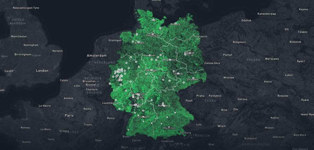
In our recent project we visualized how green German cities really are. It was the first time the interactive team of the Berliner Morgenpost used satellite imagery for a data visualization. In this post I will explain how we made use of Google Earth Engine to calculate the data and used it in order to create an interactive map application.

The Technology

Google Earth Engine is a platform that enables you to analyse petabytes of satellite images on Google's server infrastructure. You can use the web-based code editor or the Python API. It's open for scientists, researchers and developers. If you are interested in working with it you can request access. A famous application that is built with Earth Engine is Global Forest Watch, a project that keeps track of tree cover changes around the world. If you are interested in space journalism in general and also want to check out other ways on how to process satellite images, Brian T. Jacobs created an extensive list "Storytelling from Space: Tools/Resources".

Green Cities Project

Many cities in Germany claim to be the country's greenest city. There are different rankings about how green German cities are. These rankings are based on park and forest areas. We wanted to find out how green the cities really are. Therefore, in this project we analysed 185 Landsat-5, -7, and -8 images between 2005 and 2015 that have a resolution of 30x30m. Based on these images we calculated the NDVI to measure the vegetation within the official city borders. The advantage of this approach is that not only parks and forests are taken into account, but also gardens, single trees and smaller green areas. Just everything you can see on the satellite images.

Other examples for journalistic projects that use satellite images are "Loosing Ground" by Pro Publica or "Raqqa" by The New York Times.

Getting Started With Earth Engine

In the following part I will explain the script that we wrote to calculate the data and to create the image of the colored map. We used the web-based code editor for this project. In the beginning I struggled a bit with using only Earth Engine objects. These objects get handled on the server. All calculations you do in your scripts should happen on the server and not on the client. A good way to understand the basics is the Client Vs. Server section in the Developer's Guide.

Loading Data

With Earth Engine you can easily load data stored in Fusion Tables. In our case we had to load the shape of Germany and the different ones of the cities:

var germany = ee.FeatureCollection(
  'ft:1KDrYXBDlAx1fhcfmWRx7u_qqN2O_gwBNInjnGmnZ'
);
var cities = ee.FeatureCollection(
  'ft:1w4PgU3okfzwKFEIpH32oPMlOtei6hUWa9tkXv5Rt'
);

The Fusion Table with the polygons of the cities also containes data about the cities themselfes, like the names, population and the state they are in. FeatureCollections have helper methods to aggregate, sort or filter data and many more.

Using Landsat Images

You can use a lot of different data sets of the public catalogue. There are satellite images from Landsat or Sentinel but also geopysical, climate or demographic data sets you can work with. We decided to work with Landsat imagery because it provides images from a period of more than 30 years and the resolution with 30x30m was enough for our use case. The images we used in our application were shot between 2005 and 2015. We created a FeatureCollection as a kind of lookup for the Landsat ImageCollections we wanted to use for our calculations:

var landsats = ee.FeatureCollection([
  // we don't store geometry (null), only the properties (collection, nir, red, from and to) we need
  ee.Feature(null, {
    collection: ee.ImageCollection('LANDSAT/LT5_L1T_TOA'),
    nir: 'B4',
    red: 'B3',
    from: 1984,
    to: 1992,
  }),
  ee.Feature(null, {
    collection: ee.ImageCollection('LANDSAT/LT4_L1T_TOA'),
    nir: 'B4',
    red: 'B3',
    from: 1992,
    to: 1994,
  }),
  ee.Feature(null, {
    collection: ee.ImageCollection('LANDSAT/LT5_L1T_TOA'),
    nir: 'B4',
    red: 'B3',
    from: 1994,
    to: 1999,
  }),
  ee.Feature(null, {
    collection: ee.ImageCollection('LANDSAT/LE7_L1T_TOA'),
    nir: 'B4',
    red: 'B3',
    from: 1999,
    to: 2003,
  }),
  ee.Feature(null, {
    collection: ee.ImageCollection('LANDSAT/LT5_L1T_TOA'),
    nir: 'B4',
    red: 'B3',
    from: 2003,
    to: 2012,
  }),
  ee.Feature(null, {
    collection: ee.ImageCollection('LANDSAT/LE7_L1T_TOA'),
    nir: 'B4',
    red: 'B3',
    from: 2012,
    to: 2013,
  }),
  ee.Feature(null, {
    collection: ee.ImageCollection('LANDSAT/LC8_L1T_TOA'),
    nir: 'B5',
    red: 'B4',
    from: 2013,
    to: 2016,
  }),
]);

The properties are the ImageCollection, the names of the bands we need for the calculation of the NDVI (near infrared and red) and the time range (from - to) where the satellite was active. We then wrote a helper function that returns the matching Landsat data for the passed year:

Update: Because of the API changes the filter function needs to be rewritten like this:

function getLandsatByYear(year) {
  return (
    landsats
      .filter(
        ee.Filter.and(
          // filter where passed year is lower than or equal 'from' property
          ee.Filter.lte('from', year),
          // and filter where passed year is greater than 'to' property
          ee.Filter.gt('to', year)
        )
      )
      // return first matching in order to return a single object
      .first()
  );
}

There is a good overview of the different bands of the Landsat 8 you can check out, if you are interested.

Creating An Image Collection

For our analysis we had to create an image collection that only contains the images we could really use in our application. We had to filter the different Landsat collections by:

bounds - Only the area of Germany
time range - Only the vegetation-rich months june and july of the years 2005 - 2015
cloud cover - Only images with less than 5% clouds

Fortunately the ImageCollection object has functions like filterBounds, filterDate or filterMetadata to do this:

var accumulateImages = function (year, imageCollection) {
  // eg. 2006-06-01
  var startDate = ee.Date(ee.String(ee.Number(year).toInt()).cat(startDay));
  // eg. 2006-07-31
  var endDate = ee.Date(ee.String(ee.Number(year).toInt()).cat(endDay));
  var landsat = getLandsatByYear(year);

  // a collection of images for the passed year and an added ndvi band
  var ndviCollection = ee
    .ImageCollection(landsat.get('collection'))
    .filterBounds(germany)
    .filterDate(startDate, endDate)
    .filterMetadata('CLOUD_COVER', 'less_than', cloudCoverMax)
    .map(addNDVI(landsat));

  return ee.ImageCollection(imageCollection).merge(ndviCollection);
};

We then iterated over a list containing the years between and 2005 and 2015 and used the function above to accumulate our filtered image collection (resultCollection).

var yearList = ee.List.sequence(2005, 2015);
var resultCollection = yearList.iterate(
  accumulateImages,
  ee.ImageCollection([])
);

As you can see in the accumulateImages we also used a function called addNDVI. In this function we add a new band to every image in our collection. It is the band that holds the ndvi values for every pixel in the images:

function addNDVI(landsat) {
  return function (image) {
    return image.addBands(
      image
        .normalizedDifference([landsat.get('nir'), landsat.get('red')])
        .rename('ndvi')
    );
  };
}

We used the normalizedDifference function of the Image object to calculate the NDVI. You could also do the calculation on your own like this:

var red = image.select('B3');
var nearInfrared = image.select('B4');

image.addBands(
  nearInfrared.subtract(red).divide(nearInfrared.add(red))
).rename('ndvi'));

A Green Amount Value For Every City

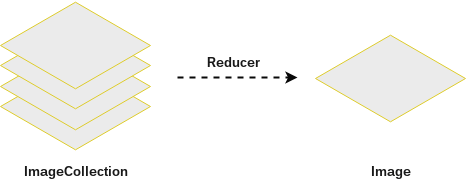
In our final application we wanted to assign a rank to the vegetation amount of every city. Therefore we had to create one image based on our ImageCollection which we can use to calculate our result. For creating the final image we used the median reducer. This reducer takes all pixels of the images inside the ImageCollection that are on top of each other and creates a new median pixel:

var resultCollectionReduced = ee
  .ImageCollection(resultCollection)
  .select('ndvi')
  .reduce(ee.Reducer.median());

You can select a certain band (in this case the "ndvi" band) of the ImageCollection and than use a reducer. There are different reducers like "min", "max", "sum" or "median", the one we used.

After this operation we have a NDVI value for every pixel in our image. We can now count the pixels inside the city borders and then calculate the amount of vegetation. We took a NDVI threshold of 0.45, so every pixel that has a NDVI which is equal or greater that 0.45 has vegetation and everything below doesn't. We did this with the following function:

function addGreenamount(ndviReduced, threshold, feature) {
  var ndviAll = ndviReduced.gte(-1);
  var ndviHigh = ndviReduced.gte(threshold);

  // count all pixels
  var allReducedSum = ndviAll.reduceRegion({
    reducer: ee.Reducer.sum(),
    geometry: feature.geometry(),
    scale: 30,
  });

  // count all pixels with an NDVI value >= passed threshold
  var partReducedSum = ndviHigh.reduceRegion({
    reducer: ee.Reducer.sum(),
    geometry: feature.geometry(),
    scale: 30,
  });

  var value_all = ee.Number(allReducedSum.get('ndvi_median'));
  var value_high = ee.Number(partReducedSum.get('ndvi_median'));

  // return amount of pixels with a NDVI value >= passed threshold
  return value_high.divide(value_all).multiply(100);
}

We can now call this function on all the cities in our FeatureCollection and add a new property "greenamount" to every feature that gets returned by the addGreenamount function.

cities = cities.map(function (feature) {
  return feature.set(
    'greenamount',
    addGreenamount(resultCollectionReduced, 0.45, feature)
  );
});

Exporting The Results

In our case we needed a colored image of the NDVI values for our visualization and the polygons of the cities with the added vegetation amounts. For the image export we have to create a RGB image. For this we take the final image and use the native visualize function. Then we can export it with the Earth Engine Export function:

Update: Because of the API changes the export function needs to be rewritten like this:

Export.image.toDrive({
  image: ndviRGB,
  description: 'germany_ndvi',
  folder: 'folder_name',
  scale: 30,
  region: germany.geometry(),
  maxPixels: 130000000000,
});

This creates a TIF image and stores it in your Google Drive account. We had to increase the maxPixels number because of the large area we wanted to export. In order to export the cities with the belonging data we used the GeoJSON export:

Export.table(cities, 'greencities_export', { fileFormat: 'GeoJSON' });

You can also export CSV, KML, or KMZ with the Export.table function. As I just saw the function we are using in our script is now deprecated and you should use this one instead:

Export.table.toDrive({
  collection: cities,
  description: 'greencities_export',
  fileFormat: 'GeoJSON',
});

If you have any questions you can contact me on twitter or use the comment section below.